
In my last post, I gave an overview of my model for the location of taxi cab drop offs in NYC. The Poisson regression used in that model isn’t the most common, and there aren’t a lot of internet resources on the technique it uses, Poisson regression. I think that this taxi cab data provides a decent example to explain Poisson regression, so I’m going to to explain how Poisson regression works, and how it can be used to understand this data.
A Recap
In my last post, I figured out the number of taxi cab drop-offs that occurred in each census tract in NYC. I found that per-capita income looks like a very promising predictor of the number of drop-offs, so I’d like to figure out how the number of drop-offs in a census tract relates to the income of that census tract.
For the sake of simplicity, I’m going to focus on using just per-capita income as a predictor of drop-offs. I plotted those values against each other in log-log space below.
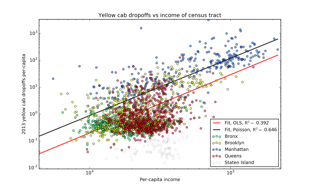 Since things look fairly linear, our initial thought would be to turn to our old friend ordinary least squares regression.
If you look at the ordinary least squares regression line though, you’ll notice something is a bit off.
While there is clearly a linear relationship in log-log space, the regression line doesn’t follow it at all.
Since things look fairly linear, our initial thought would be to turn to our old friend ordinary least squares regression.
If you look at the ordinary least squares regression line though, you’ll notice something is a bit off.
While there is clearly a linear relationship in log-log space, the regression line doesn’t follow it at all.
We can think about regression as having two parts. The most familiar part is the prediction for the mean. This is the predicted line that we can plot. The second part is the “random part” of the model. The model expects that the mean will not perfectly predict all the data. While ordinary least squares doesn’t necessarily choose a specific distribution, it does assume that the variance is constant1.
However, for our taxi cab data, this is not the case. If you were to count the number of taxi cab drop offs in a bunch of identical census tracts, the data wouldn’t be normally distributed. Instead, like most count data, it would follow a Poisson distribution. The variance of a Poisson distribution is not constant, but is equal to the mean. This means that we’re going to have to turn to a slightly different regression method to understand this data. As it will assume the data have a Poisson distribution about the mean, it’s called Poisson regression.
Building Poisson Regression from the Distribution Up
In order to build this regression method, we’ll start with what we know: the Poisson distribution probability density function: \[p(y,\lambda) = \frac{\lambda^y e^{-\lambda}}{y !},\] where \(y\) is the sample, and \(\lambda\) is the mean. For our model, we’re going to assume that the mean is some function of the independent variables \(\mathbf{x}\) and the parameters that we’re going to fit, \(\boldsymbol{\theta}\). Using this, the probability of finding the data point \( y_i \) given values for the independent variables \(\mathbf{x}_i\) is \[p\left(y_i|\lambda\left(\mathbf{x}_i,\boldsymbol{\theta}\right)\right) = \frac{\lambda\left(\mathbf{x}_i,\boldsymbol{\theta}\right)^{y_i} e^{-\lambda\left(\mathbf{x}_i,\boldsymbol{\theta}\right)}}{y_i !}\] Then, the probability of getting all the data is just the product of all the data probabilities multiplied together. \[L(y_i,\lambda\left(\mathbf{x}_i,\boldsymbol{\theta}\right)) = \prod_{i=0}^N \frac{\lambda\left(\mathbf{x}_i,\boldsymbol{\theta}\right)^{y_i} e^{-\lambda\left(\mathbf{x}_i,\boldsymbol{\theta}\right)}}{y_i !}\] This function is called the likelihood function. Our regression method will simply find the values of the parameters \(\boldsymbol{\theta}\) that maximize this likelihood function. These parameters will be the parameters under which our data is the most probable.
In practice though, maximizing a bunch of products like this can be a little difficult. We can make our lives easier by taking the logarithm of both sides. Since \(a > b \implies \log (a) > \log (b)\), the values of \(\boldsymbol{\theta}\) that maximize the log of the likelihood - called the log-likelihood - will also maximize the likelihood itself.
Taking the log of the likelihood gives us a summation to minimize instead of a product: \[\log(L(y,\lambda\left(\mathbf{x},\boldsymbol{\theta}\right))) = l(y,\lambda\left(\mathbf{x},\boldsymbol{\theta}\right)) = \sum_{i=0}^N y_i \log(\lambda\left(\mathbf{x}_i,\boldsymbol{\theta}\right)) - \lambda\left(\mathbf{x}_i,\boldsymbol{\theta}\right) - \log(y_i !)\] Finding the maximum of \(l(y,\lambda\left(\mathbf{x},\boldsymbol{\theta}\right))\) is still not super easy. In practice, we’re going to have a computer find the maximum for us. There are a bunch of different algorithms we could use, as optimization problems like these are very common.
Choosing a form for the mean
Now we need to choose a functional form for the mean, \(\lambda\left(\mathbf{x}_i,\boldsymbol{\theta}\right)\). We noticed before that things looked linear when we looked at the log of the per capita drop offs, so we’ll use a log in our functional form. Taking the log is actually the most common choice for count data. As logs can’t go negative, we won’t make negative predictions for counts which don’t make sense. We’ll assume that the log of per-capita counts behaves linearly, so \[ \log \left(\frac{\lambda_i}{c_i}\right) = \boldsymbol{\theta} \cdot \mathbf{x}_i + k,\] where \(c_i\) is the population for the \(i\)-th census tract, \(\frac{\lambda_i}{c_i}\) is the drop offs per-capita, and \(k\) is a constant. The functional form for \(\lambda\left(\mathbf{x}_i,\boldsymbol{\theta}\right)\) is then \[ \lambda\left(\mathbf{x}_i,\boldsymbol{\theta}\right) = c_i \exp(\boldsymbol{\theta} \cdot \mathbf{x}_i + k). \] We can plug this into our log-likelihood to get the log-likelihood of our specific model, \[ l(y,\mathbf{x},\boldsymbol{\theta}) = \sum_{i=0}^N y_i \left[\boldsymbol{\theta} \cdot \mathbf{x}_i + k + \log\left(c_i\right) \right] -c_i \exp(\boldsymbol{\theta} \cdot \mathbf{x}_i + k) - \log(y_i !) \]
Fit it!
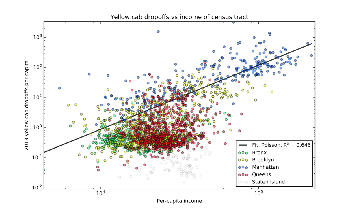
The fit for this model, using just the log of income as a predictor, looks pretty good based on the highly technical “just eyeball it” test. But we really ought to be able to quantify how well we’ve done. With OLS, we would probably look at the \(R^2\) value. But for our data, this isn’t a great idea. Since the variance of a Poisson distribution is equal to the mean, we’d expect the variance to be a lot higher for higher predictions, and we’d get penalized a lot more for them then the rest of the data. A better approach is to come up with some quantities from the likelihood function we calculated. We can compare the likelihood we got to the likelihood we would get with a similar model that gets the means exactly on the data. We look at the ratio of the squares of the two likelihoods, \[ \left[\frac{L(y,y)}{L(y,\lambda\left(\mathbf{x}_i,\boldsymbol{\theta}\right))}\right]^2 \] Since we’re usually working with the log-likelihood, we’ll take the logs and look at that: \[ D(y, \lambda\left(\mathbf{x}_i,\boldsymbol{\theta}\right))) = 2 l(y,y) - 2 l (y, \lambda\left(\mathbf{x}_i,\boldsymbol{\theta}\right))). \] This is called the deviance. Conceptually, it represents a sort of distance between the perfect model and the model we’re testing. It also will be drawn from a \(\chi^2\) distribution and we can derive p-values from it.
For the model I created of the taxi cabs, we find a deviance of \(2 \times 10^8\), which gives a p-value of 0. Note that this p-value is a bit different from the most common set up. Since the perfect model is the more complex of the two models, our model is in the place of the null hypothesis. This seems pretty disastrous for our model.
However, we shouldn’t be that surprised. What this indicates is that there are other factors involved with taxi cab drop offs that we haven’t accounted for.
In ordinary least squares, the effect of these factors would show up in a high variance for our model. But since the random part of our model is a Poisson distribution, the variance is always equal to the mean. If our model actually described everything involved, than this wouldn’t be a problem, as we’d know the mean exactly. However, we don’t. There are clearly other factors involved in taxicab drop offs, and we can’t hope to build a model with all of them. Thus, we have more variance than expected, a situation called overdispersion. Since we think that the assumption that the variance will be equal to the mean isn’t a good one, we can relax this assumption. Instead, we’ll build a model where the variance is equal to a constant times the mean. The way we will do this is a bit of an inelegant hack though. The Poisson distribution is strictly larger than zero, so we don’t really have room to just widen the distribution, as that would push it below zero. Thus, we can’t create a real distribution that the random component of our model will follow with the right properties. Instead, we create a model that doesn’t have a real distribution behind it at all. It’s just something that looks a lot like a Poisson regression, except for the larger variance. This is done by modifying the log-likelihood that we created for Poisson regression. The log-likelihood we create - called a quasi-log-likelihood - is \[ l(y,\lambda\left(\mathbf{x},\boldsymbol{\theta}\right)) = \sum_{i=0}^N \frac{y_i \log(\lambda\left(\mathbf{x}_i,\boldsymbol{\theta}\right)) - \lambda\left(\mathbf{x}_i,\boldsymbol{\theta}\right)}{\sigma^2} \] \(\sigma^2\) is the factor by which our variance is increased, called the dispersion parameter. This model is called a quasi-Poisson regression. If you compare this quasi-log-likelihood to the true Poisson regression log-likelihood, you’ll notice that they’re pretty similar. As far as finding the parameters \(\boldsymbol{\theta}\) go, they are identical, as for both, \[ \frac{\partial l(y,\lambda\left(\mathbf{x},\boldsymbol{\theta}\right))}{\partial \boldsymbol{\theta}} = \mathbf{0} \implies \sum_{i=0}^N \left[ \frac{y_i}{\lambda\left(\mathbf{x}_i,\boldsymbol{\theta}\right)} - 1 \right] \frac{\partial \lambda\left(\mathbf{x}_i,\boldsymbol{\theta}\right)}{\partial \boldsymbol{\theta}} = \mathbf{0}. \]
Thus, the model for the mean will be identical for both models. However, with a scaling factor on the log-likelihood, the random part of the quasi-Poisson model has a larger variance than the ordinary Poisson, so things like p-values and the confidence intervals will be changed.
While quasi-Poisson regression might be inelegant, it is generally the rule rather than the exception with real data. It’s rare that you can build a model where you can perfectly model the mean, so there will be some unexplained variance and the quasi-Poisson model is required.
Under the quasi-Poisson model, our p-value is increased to one, and we can accept our hypothesis. This should be taken with a grain of salt though. The dispersion parameter itself is a measure of how much the data is spread our compared to what we’d expect from ordinary Poisson regression. The dispersion parameter we find for our model is \(5\times10^2\). This indicates that there is a lot of variance that can be further explained.
How good is the random component
But how well does the random component explain the data?
Does the data actually follow a Poisson distribution - or at least the wider version of it we created for quasi-Poisson regression?
For ordinary least squares, we’d usually plot the quantiles of the residuals against that of a normal distribution to see if they follow a normal distribution.
But we can’t do the same with a Poisson distribution.
Since the Poisson distribution changes with the mean, each residual is drawn from a different distribution.
We can get around this by transforming the residuals such that they should follow a normal distribution, if they actually are following our model.
For Poisson regression, these Anscombe residuals are given by
\[
r_A = \frac{3\left(y^{2/3} - \lambda ^{2/3}\right)}{2\lambda^{1/6}}.
\]
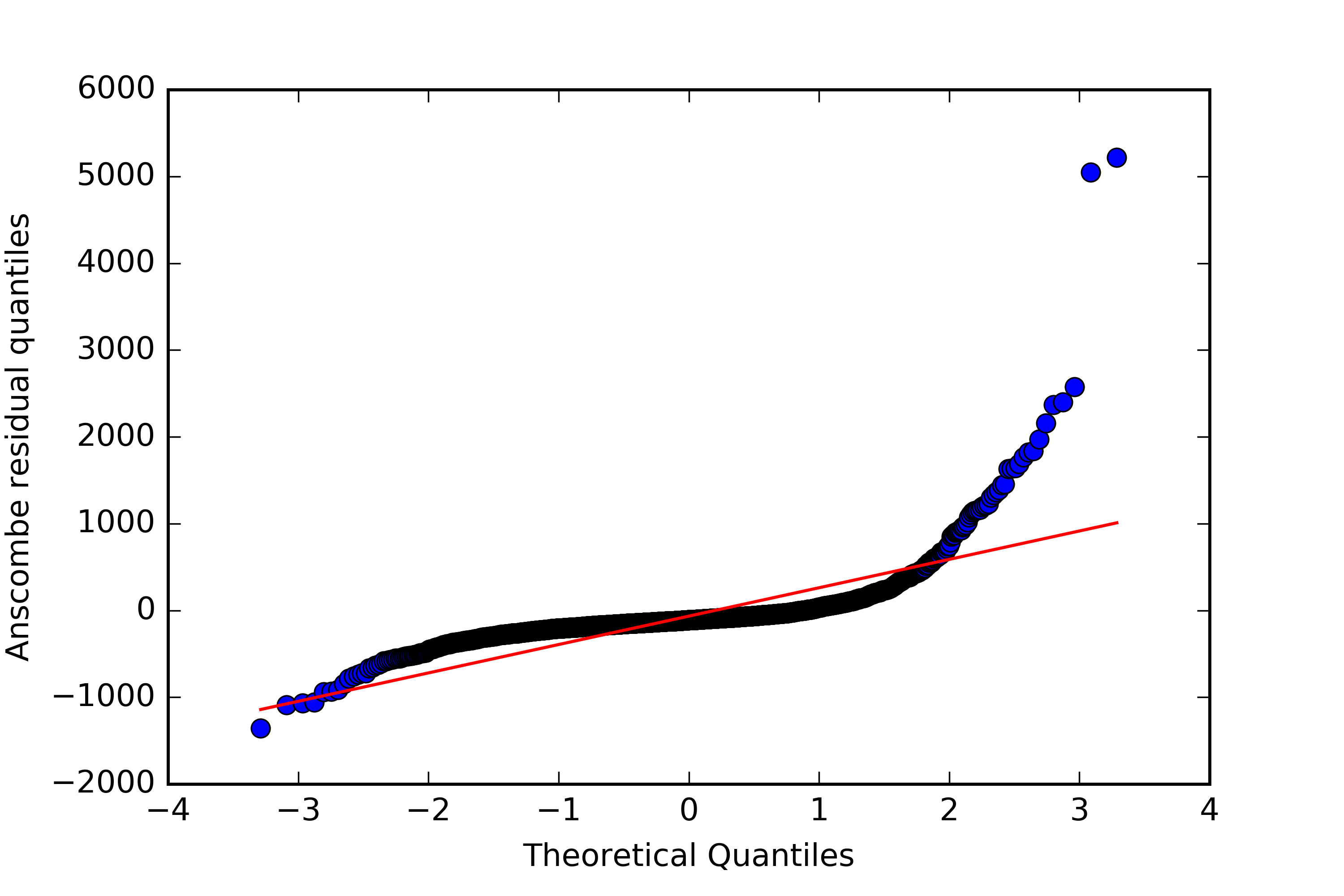 We can compute these residuals for our data, and see if they follow the normal distribution as predicted.
Unsurprisingly, given the fact that we had to dramatically adjust our variance, the distribution isn’t that close to normal.
It’s generally more narrow around the mean, with relatively longer tails that that of a normal distribution.
We can compute these residuals for our data, and see if they follow the normal distribution as predicted.
Unsurprisingly, given the fact that we had to dramatically adjust our variance, the distribution isn’t that close to normal.
It’s generally more narrow around the mean, with relatively longer tails that that of a normal distribution.
\(R^2\)
The deviance doesn’t quite capture the same thing that a quantity like \(R^2\) does. We’d like a value that give a measure of explained variance vs a model that just predicts a constant value (the null model). There are a couple of ways to do this, none of which cover all the bases that \(R^2\) does. I’m going to focus on one that gives a good measure of explained variance. It’s built on the log-likelihood we already computed, and is given by \[ R^2 = 1- \frac{l(y, \lambda(\mathbf{x},\boldsymbol{\theta}))}{l(y,\bar{y})}. \] In this equation, \(l(y,\bar{y})\) represents the log-likelihood of the null model, where all data points are assumed to be drawn from a Poisson distribution with a mean of \(\bar{y}\). It’s also important to note that the log-likelihood is always negative. Since the likelihood is a probability that ranges from 0 to 1, the log of it will always be negative. While we expect \(l(y, \bar{y})\) to be smaller than \(l(y, \lambda(\mathbf{x},\boldsymbol{\theta}))\), since they are negative, the absolute value of \(l(y, \bar{y})\) will be larger. The maximum theoretical value for a log-likelihood is thus 0, so the maximum value for the psuedo-\(R^2\) we defined is 1, just like a true \(R^2\). For our data, we find an impressively high value of 0.65. This means that there is a very large amount of explained variance with our model, and that it is a dramatic improvement over the null model.
Conclusion
Based on the metrics I went into here, this model is a mixed bag. Per-capita income is an impressive predictor for taxicab drop-offs, with a pseudo-\(R^2\) of 0.65. However, the high dispersion parameter, along with the poor fit of the Anscombe residuals to a normal distribution indicates that there are still many other factors contributing to the number of drop offs. I explored some of the demographic factors available from the Census Bureau, but none significantly increased the pseudo-\(R^2\) that much. Income may be an especially hard predictor to beat because it correlates well with many other factors that might be more directly causing lots of drop offs. Having a lot of popular taxi destinations, like jobs, stores, and restaurants, will generally make an area attractive to residents and increase housing prices. Increased housing prices will force out low income residents and bring in high income residents, bringing The Census Bureau also publishes data on commercial activity split up by zip code, such as the number of people working there. Unfortunately, zip codes, especially in Manhattan, cross census tracts in complicated ways, and it’s going to be time intensive to sift through the data.
A good additional predictor should lower the dispersion parameter and bring the Anscombe residuals closer to normal. This could come from very different sources, as the Anscombe residuals are mostly off on the high and low extreme values of our data. It could be that there are some very specific reasons for the small number of census tracts that are on the margins to be off.
There are some other methods of model verification that I didn’t go over here, such as the Wald test, and there are a bunch of other types of residuals and transformed residuals that have specific purposes for analyzing a model, enough to fill a whole textbook. In fact, there is a whole, excellent textbook on the subject of Poisson regression and other regression methods that can be built from the maximum likelihood estimation I used here. It’s called Generalized Linear Models, by McCullagh and Nelder. It’s been around for a while, and a google search will turn up a bunch of digital versions.
1 Most derivations of ordinary least squares don’t assume any specific distribution. Using the maximum likelihood method that I described here, you could create a linear regression model that assumes a normal distribution of the residuals. This model will be equivalent to ordinary least squares. In fact, if you create a regression model with any distribution with constant variance, you will end up with ordinary least squares.